Preliminaries

Libraries for data processing —
```
library("dplyr")
library("tidyr")
```

Libraries for plotting —

library("ggplot2")
library("gridExtra")
library("scales")

Libraries for financial data —

library("quantmod")
library("GLDEX")
library("MASS")

User defined functions —

source("./scripts/my_functions_returns.R")

Introduction

We will look at data of three broad market indices to get an idea of the movements of the market as a whole and obtain distributions/statistics to use in the Rent vs. Buy application as the basis of the simulated market returns.

This analysis was motivated by two interesting blog posts:

The GLDEX package is available on CRAN.

Three Broad Market Indices : Daily Returns

The three indices we study are:

Vanguard Total Stock Market Index (VTSMX),
S&P 500 (^GSPC)
NASDAQ 100 (^NDX)

Returns

We consider two (obviously related) quantities expressing the return of an asset described by an ordered set of values \({x_i}\):

log return: \[ {rl}_i = \log\left(\frac{x_i}{x_{i-1}}\right) \]
relative return: \[ {rr}_i = e^{rl_i} - 1 = \frac{x_i - x_{i-1}}{x_{i-1}} \]

Setup

start.date <- "1986-01-01"
end.date <- "2014-12-31"

xxlin <- seq(-25.0, 25.0, by = 0.1)
xxlog <- seq(-2.0, 2.0, by = 0.001)

Vanguard Total Stock Market Index

Fetch the data with quantmod:

# getSymbols("VTSMX", from = "1994-01-01")
getSymbols("VTSMX", from = start.date, to = end.date)
# [1] "VTSMX"
VTSMX.vec <- as.vector(VTSMX[, 4])

Prepare returns:

VT <- prepare_data(data = VTSMX.vec, xlin = xxlin, xlog = xxlog)

VT$dates <- index(VTSMX)
VT$year <- substr(index(VTSMX), 1, 4)

The function prepare_data() returns a list with (for each rr and rl): the data themselves, parameters of the best fit with the generalized Gamma distribution, distributions for this latter and two Gaussians fit to the data in two narrow (less than \(\sigma\) wide) ranges around the mean.
We add to this list dates from the timeseries index and year:

This is the structure of the resulting list:

str(VT)
# List of 12
#  $ rr_data  : num [1:5714] -0.299 0 1.8 0 0.688 ...
#  $ rr_fit_gl: num [1:4] 0.077 2.552 -0.279 -0.218
#  $ rr_fit_n1: Named num [1:2] 0.0402 1.0624
#   ..- attr(*, "names")= chr [1:2] "mean" "sd"
#  $ rr_fit_n2: Named num [1:2] 0.0586 0.7716
#   ..- attr(*, "names")= chr [1:2] "mean" "sd"
#  $ rr_distr :'data.frame':    501 obs. of  4 variables:
#   ..$ x      : num [1:501] -25 -24.9 -24.8 -24.7 -24.6 -24.5 -24.4 -24.3 -24.2 -24.1 ...
#   ..$ y_gl   : num [1:501] 0.0000036 0.00000367 0.00000373 0.0000038 0.00000386 ...
#   ..$ y_norm1: num [1:501] 8.96e-122 8.20e-121 7.44e-120 6.68e-119 5.96e-118 ...
#   ..$ y_norm2: num [1:501] 4.77e-230 3.19e-228 2.09e-226 1.35e-224 8.56e-223 ...
#  $ rl_data  : num [1:5714] -0.003 0 0.01784 0 0.00685 ...
#  $ rl_fit_gl: num [1:4] 0.000784 255.660582 -0.285599 -0.212883
#  $ rl_fit_n1: Named num [1:2] 0.000381 0.010626
#   ..- attr(*, "names")= chr [1:2] "mean" "sd"
#  $ rl_fit_n2: Named num [1:2] 0.000575 0.007711
#   ..- attr(*, "names")= chr [1:2] "mean" "sd"
#  $ rl_distr :'data.frame':    4001 obs. of  4 variables:
#   ..$ x      : num [1:4001] -2 -2 -2 -2 -2 ...
#   ..$ y_gl   : num [1:4001] 0.0000000436 0.0000000437 0.0000000438 0.0000000439 0.0000000441 ...
#   ..$ y_norm1: num [1:4001] 0 0 0 0 0 0 0 0 0 0 ...
#   ..$ y_norm2: num [1:4001] 0 0 0 0 0 0 0 0 0 0 ...
#  $ dates    : Date[1:5715], format: "1992-04-27" "1992-04-28" "1992-04-29" ...
#  $ year     : chr [1:5715] "1992" "1992" "1992" "1992" ...

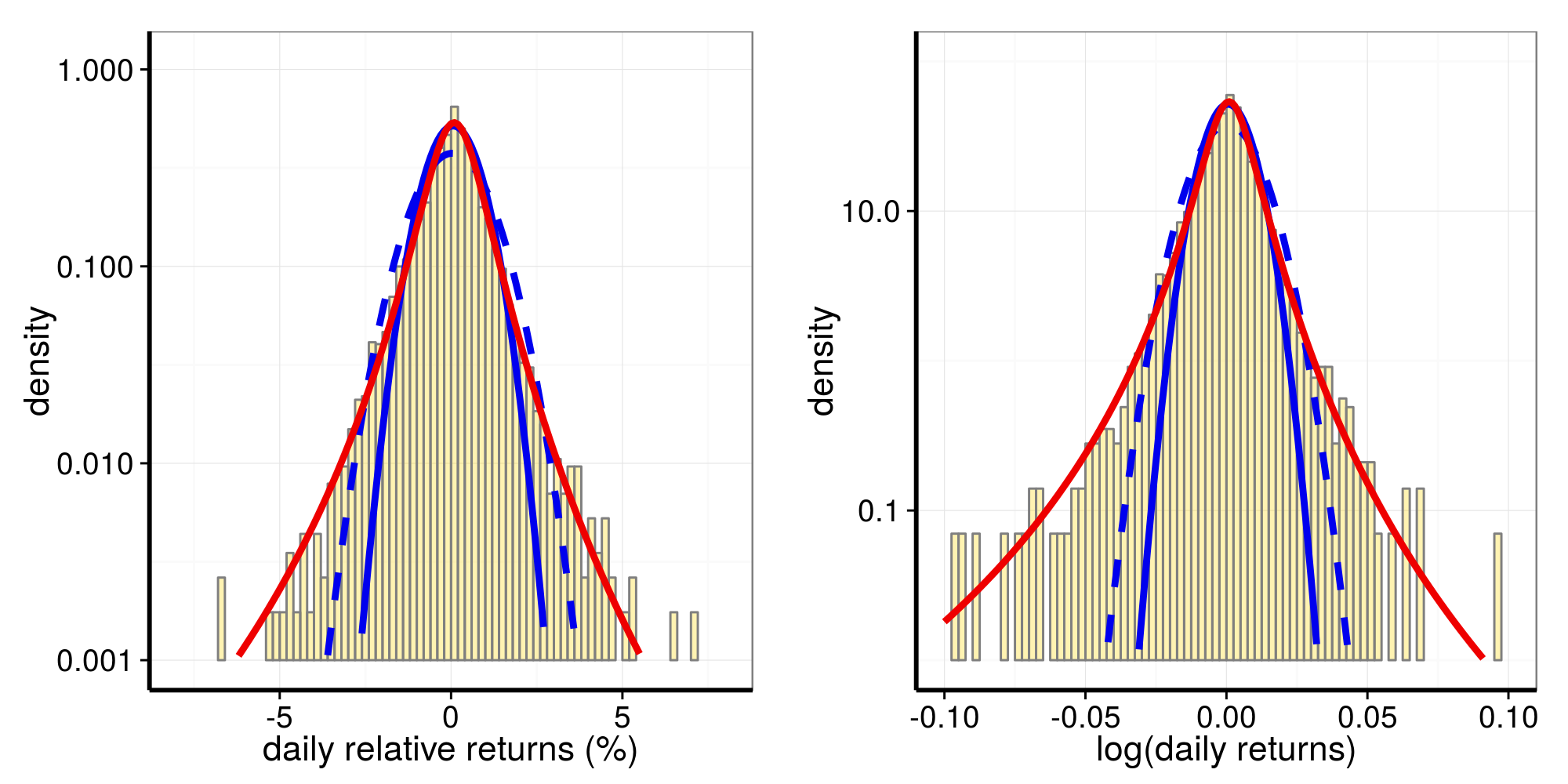
Distributions of relative returns and of log returns:

The histograms are the return data, with overlayed

in red the generalized Gamma distribution, and
in blue the two Gaussians fit to the “core” of the data.

It is quite obvious how much better the generalized Gamma distribution describes the data, both their “code” and the long fat tails.

S&P 500

Some treatment as the VTSMX data.

Fetch the data with quantmod:

getSymbols("^GSPC", from = start.date, to = end.date)
# [1] "GSPC"
GSPC.vec <- as.vector(GSPC[, 4])

and prepare with the prepare_data() function:

SP <- prepare_data(data = GSPC.vec, xlin = xxlin, xlog = xxlog)

SP$dates <- index(GSPC)
SP$year <- substr(index(GSPC), 1, 4)

This is the structure of the resulting list:

str(SP)
# List of 12
#  $ rr_data  : num [1:7311] 0.615 -0.109 1.495 -2.727 -0.894 ...
#  $ rr_fit_gl: num [1:4] 0.0702 2.5498 -0.2594 -0.2118
#  $ rr_fit_n1: Named num [1:2] 0.0453 1.0377
#   ..- attr(*, "names")= chr [1:2] "mean" "sd"
#  $ rr_fit_n2: Named num [1:2] 0.0559 0.7676
#   ..- attr(*, "names")= chr [1:2] "mean" "sd"
#  $ rr_distr :'data.frame':    501 obs. of  4 variables:
#   ..$ x      : num [1:501] -25 -24.9 -24.8 -24.7 -24.6 -24.5 -24.4 -24.3 -24.2 -24.1 ...
#   ..$ y_gl   : num [1:501] 0.0000023 0.00000234 0.00000239 0.00000243 0.00000248 ...
#   ..$ y_norm1: num [1:501] 1.22e-127 1.24e-126 1.26e-125 1.26e-124 1.24e-123 ...
#   ..$ y_norm2: num [1:501] 2.10e-232 1.47e-230 1.00e-228 6.77e-227 4.49e-225 ...
#  $ rl_data  : num [1:7311] 0.00614 -0.00109 0.01484 -0.02765 -0.00898 ...
#  $ rl_fit_gl: num [1:4] 0.000714 255.280258 -0.265821 -0.206393
#  $ rl_fit_n1: Named num [1:2] 0.000433 0.010393
#   ..- attr(*, "names")= chr [1:2] "mean" "sd"
#  $ rl_fit_n2: Named num [1:2] 0.00055 0.00768
#   ..- attr(*, "names")= chr [1:2] "mean" "sd"
#  $ rl_distr :'data.frame':    4001 obs. of  4 variables:
#   ..$ x      : num [1:4001] -2 -2 -2 -2 -2 ...
#   ..$ y_gl   : num [1:4001] 0 0 0 0 0 0 0 0 0 0 ...
#   ..$ y_norm1: num [1:4001] 0 0 0 0 0 0 0 0 0 0 ...
#   ..$ y_norm2: num [1:4001] 0 0 0 0 0 0 0 0 0 0 ...
#  $ dates    : Date[1:7312], format: "1986-01-02" "1986-01-03" "1986-01-06" ...
#  $ year     : chr [1:7312] "1986" "1986" "1986" "1986" ...

Distributions of relative returns and of log returns:

p1 <- plot_distr_rel_returns(data = SP$rr_data, fits = SP$rr_distr)
p2 <- plot_distr_log_returns(data = SP$rl_data, fits = SP$rl_distr)
grid.arrange(p1, p2, nrow=1)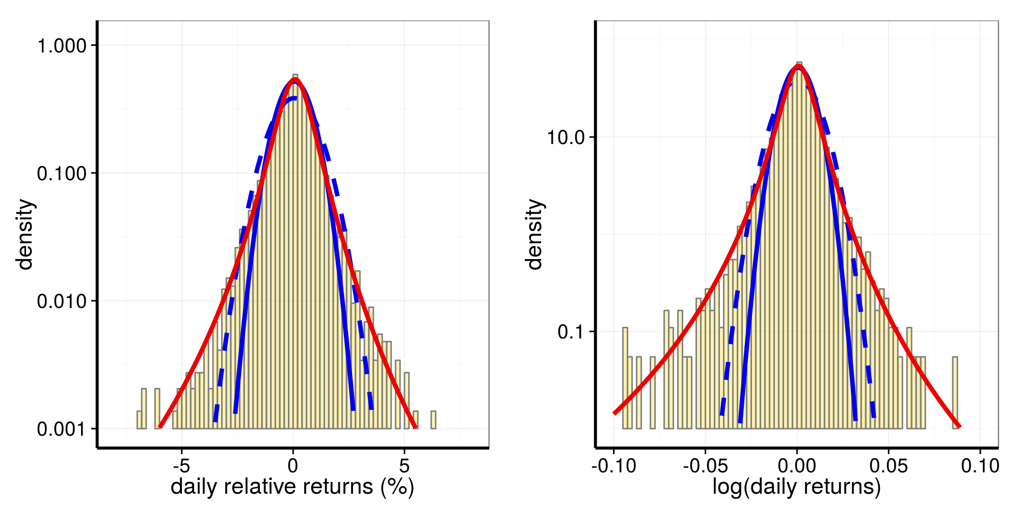

NASDAQ 100

Fetch the data with quantmod:

getSymbols("^NDX", from = start.date, to = end.date)
# [1] "NDX"
NDX.vec <- as.vector(NDX[, 4])

NN <- prepare_data(data = NDX.vec, xlin = xxlin, xlog = xxlog)

NN$dates <- index(NDX)
NN$year <- substr(index(NDX), 1, 4)

This is the structure of the resulting list:

str(NN)
# List of 12
#  $ rr_data  : num [1:7311] -0.537 -0.149 1.868 -1.227 -1.799 ...
#  $ rr_fit_gl: num [1:4] 0.113 1.68 -0.265 -0.213
#  $ rr_fit_n1: Named num [1:2] 0.0558 1.4476
#   ..- attr(*, "names")= chr [1:2] "mean" "sd"
#  $ rr_fit_n2: Named num [1:2] 0.0949 0.8966
#   ..- attr(*, "names")= chr [1:2] "mean" "sd"
#  $ rr_distr :'data.frame':    501 obs. of  4 variables:
#   ..$ x      : num [1:501] -25 -24.9 -24.8 -24.7 -24.6 -24.5 -24.4 -24.3 -24.2 -24.1 ...
#   ..$ y_gl   : num [1:501] 0.0000111 0.0000112 0.0000114 0.0000116 0.0000119 ...
#   ..$ y_norm1: num [1:501] 2.43e-66 8.01e-66 2.63e-65 8.58e-65 2.79e-64 ...
#   ..$ y_norm2: num [1:501] 3.57e-171 8.05e-170 1.79e-168 3.94e-167 8.55e-166 ...
#  $ rl_data  : num [1:7311] -0.00539 -0.00149 0.01851 -0.01235 -0.01816 ...
#  $ rl_fit_gl: num [1:4] 0.00116 168.5565 -0.27619 -0.20523
#  $ rl_fit_n1: Named num [1:2] 0.000509 0.014442
#   ..- attr(*, "names")= chr [1:2] "mean" "sd"
#  $ rl_fit_n2: Named num [1:2] 0.000915 0.008969
#   ..- attr(*, "names")= chr [1:2] "mean" "sd"
#  $ rl_distr :'data.frame':    4001 obs. of  4 variables:
#   ..$ x      : num [1:4001] -2 -2 -2 -2 -2 ...
#   ..$ y_gl   : num [1:4001] 0.000000127 0.000000127 0.000000127 0.000000128 0.000000128 ...
#   ..$ y_norm1: num [1:4001] 0 0 0 0 0 0 0 0 0 0 ...
#   ..$ y_norm2: num [1:4001] 0 0 0 0 0 0 0 0 0 0 ...
#  $ dates    : Date[1:7312], format: "1986-01-02" "1986-01-03" "1986-01-06" ...
#  $ year     : chr [1:7312] "1986" "1986" "1986" "1986" ...

Distributions of relative returns and of log returns:

p1 <- plot_distr_rel_returns(data = NN$rr_data, fits = NN$rr_distr)
p2 <- plot_distr_log_returns(data = NN$rl_data, fits = NN$rl_distr)
grid.arrange(p1, p2, nrow=1)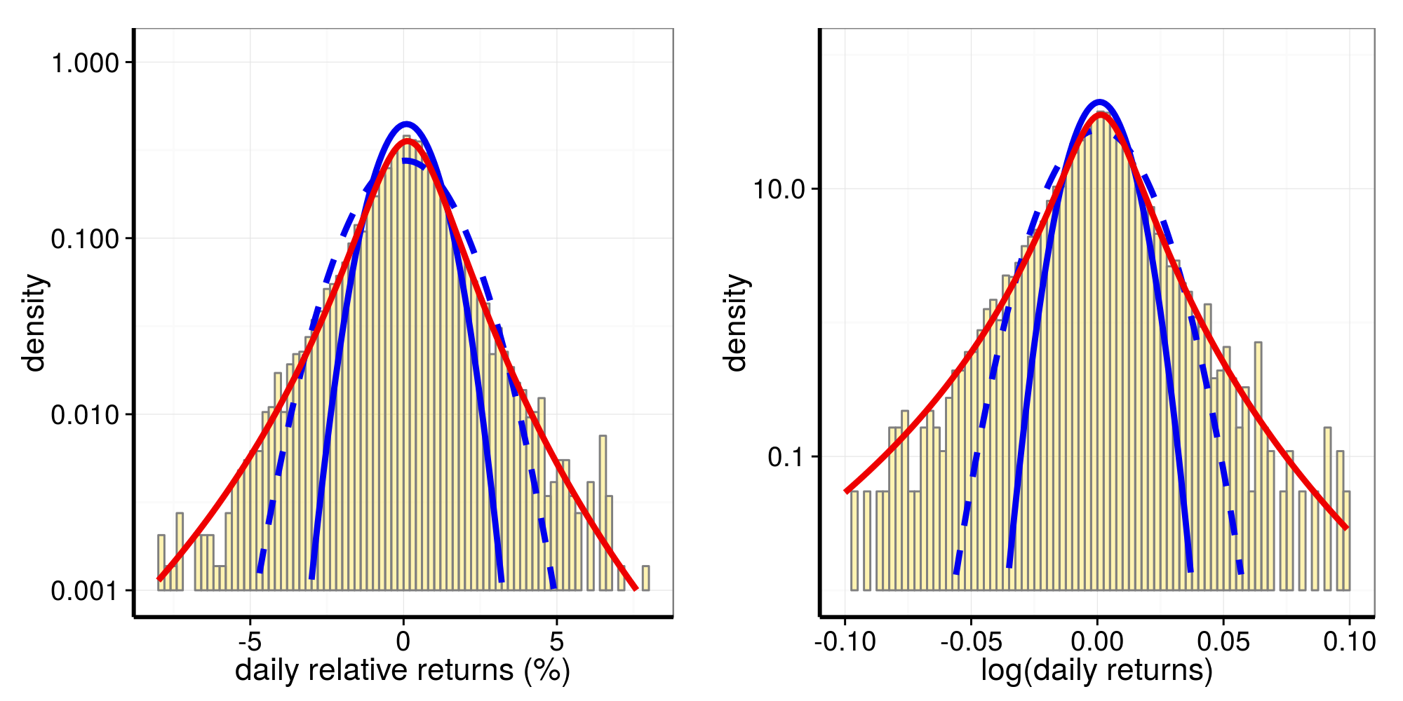

Three Broad Market Indices : Annual Returns

Annual from Daily Returns

Simulating annual returns by compounding daily returns drawn from the best fit generalized gamma distributions.

# typical number of market days in a year is ~252
ndays <- 252

# repeats
  N <- 1e5
# N <- 1e6

set.seed(1212)
test_rr.VTSMX <- rep(0, N)
for(j in 1:N) {
    dummy <- rgl(ndays, VT$rr_fit_gl)
    test_rr.VTSMX[j] <- (cumprod(1 + dummy/100)[ndays] - 1.0)*100
}

test_rr.SP500 <- rep(0, N)
for(j in 1:N) {
    dummy <- rgl(ndays, SP$rr_fit_gl)
    test_rr.SP500[j] <- (cumprod(1 + dummy/100)[ndays] - 1.0)*100
}

test_rr.N100 <- rep(0, N)
for(j in 1:N) {
    dummy <- rgl(ndays, NN$rr_fit_gl)
    test_rr.N100[j] <- (cumprod(1 + dummy/100)[ndays] - 1.0)*100
}

… and from the Gaussian best fit to the “core” of the returns distribution.

# typical number of market days in a year is ~252
ndays <- 252

# repeats
  N <- 1e5
# N <- 1e6

set.seed(1414)
test_rr_n1.VTSMX <- rep(0, N)

print(ndays)
# [1] 252
print(VT$rr_fit_n1)
#      mean        sd 
# 0.0402238 1.0624322

for(j in 1:N) {
    dummy <- rnorm(ndays, VT$rr_fit_n1)
    test_rr_n1.VTSMX[j] <- (cumprod(1 + dummy/100)[ndays] - 1.0)*100
}

test_rr_n1.SP500 <- rep(0, N)
for(j in 1:N) {
    dummy <- rnorm(ndays, SP$rr_fit_n1)
    test_rr_n1.SP500[j] <- (cumprod(1 + dummy/100)[ndays] - 1.0)*100
}

test_rr_n1.N100 <- rep(0, N)
for(j in 1:N) {
    dummy <- rnorm(ndays, NN$rr_fit_n1)
    test_rr_n1.N100[j] <- (cumprod(1 + dummy/100)[ndays] - 1.0)*100
}

xx2 <- seq(-200, 200, by = 1.0)
yy.VTSMX.n <- dnorm(xx2, mean = mean(test_rr.VTSMX), sd = sd(test_rr.VTSMX))
yy.SP500.n <- dnorm(xx2, mean = mean(test_rr.SP500), sd = sd(test_rr.SP500))
yy.N100.n  <- dnorm(xx2, mean = mean(test_rr.N100), sd = sd(test_rr.N100))

plot(density(test_rr.N100), type = "n",
     xlim = c(-100.0, 200.0), 
     ylim = c(0.0, 0.037), 
     xlab = "annual return [%]", 
     main = "VTSMX, S&P500, NASDAQ100")
grid()
lines(xx2, yy.N100.n,         col = "red2",   lwd = 3, lty = 3)
lines(xx2, yy.SP500.n,        col = "blue2",  lwd = 3, lty = 3)
lines(xx2, yy.VTSMX.n,        col = "green3", lwd = 3, lty = 3)
lines(density(test_rr.N100),  col = "red2",   lwd = 3)
lines(density(test_rr.SP500), col = "blue2",  lwd = 3)
lines(density(test_rr.VTSMX), col = "green3", lwd = 3)
legend("topleft", bty = "y", bg = "grey95", x.intersp = 0.7, y.intersp = 0.8, 
       legend = c("Nasdaq100", "S&P 500", "VTSMX"), 
       lty = 1, lwd = 3,
       col = c("red2", "blue2", "green3"),
       cex = 1.0)
legend("topright", bty = "y", bg = "grey95", x.intersp = 0.7, y.intersp = 0.8, 
       legend = c("from simulations", "Gaussian"),
       lty = c(1, 3), lwd = 3, seg.len = 4,
       col = c("grey10", "grey10"),
       cex = 1.0)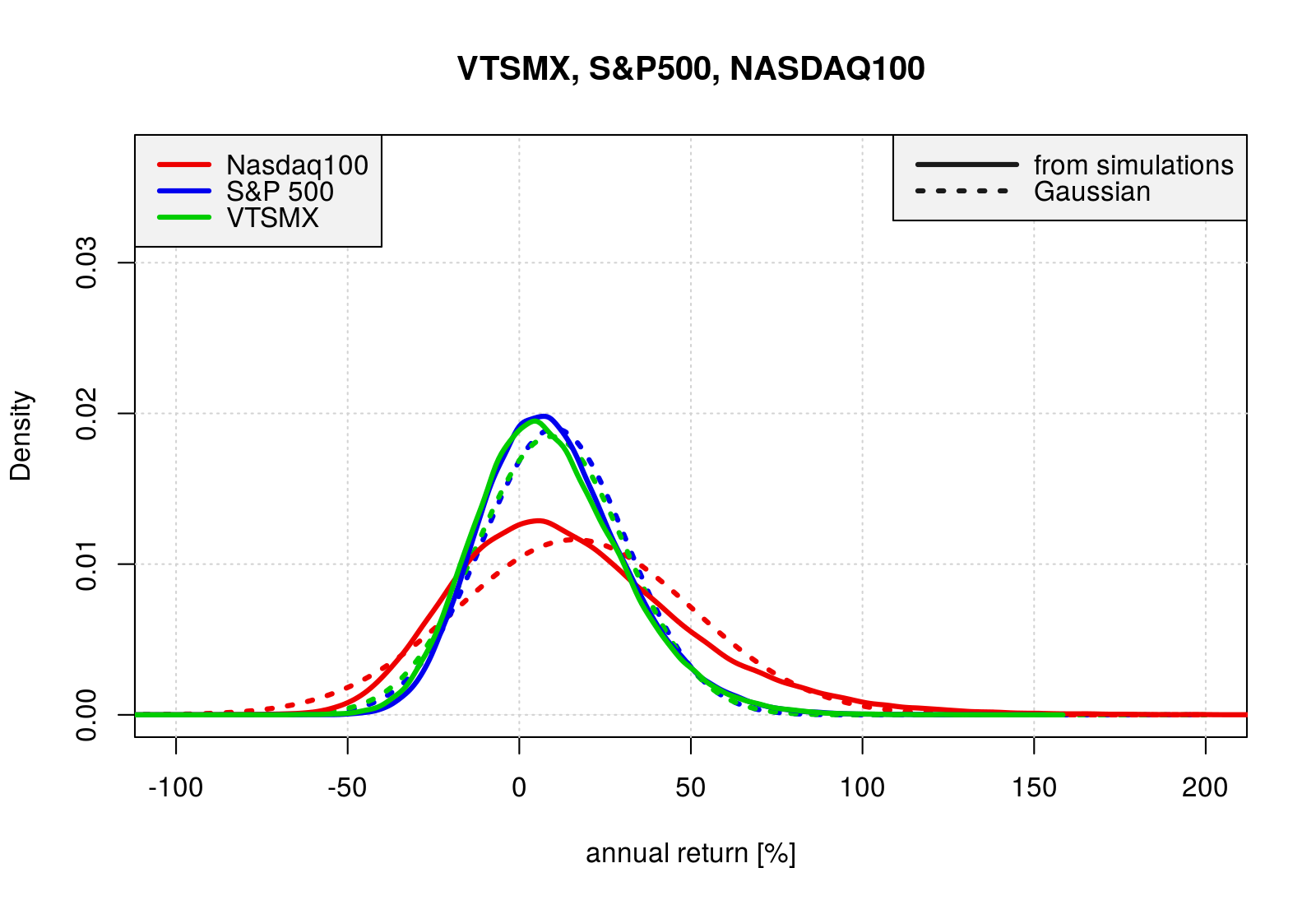

Annual straight from data

The simulated daily-compounded annual returns can be compared with a crude estimate of annual returns obtained straight from the data by looking at 252-day-lagged values.

For this analysis we restricted the data to the 1994-2014 interval, in order to have the same coverage for the three indices.

VTb <- VTSMX.vec[VT$year >= 1994]
SPb <- GSPC.vec[SP$year >= 1994]
NNb <- NDX.vec[NN$year >= 1994]
VTd <- index(VTSMX)[VT$year >= 1994]
SPd <- index(GSPC)[SP$year >= 1994]
NNd <- index(NDX)[NN$year >= 1994]

VTSMX_rla <- diff(log(VTb), lag = 252)
VTSMX_rra <- 100.0*(exp(VTSMX_rla)-1)

SP500_rla <- diff(log(SPb), lag = 252)
SP500_rra <- 100.0*(exp(SP500_rla)-1)

N100_rla <- diff(log(NNb), lag = 252)
N100_rra <- 100.0*(exp(N100_rla)-1)

rr.df <- data.frame(date = VTd[-(1:252)], VT = VTSMX_rra, SP = SP500_rra, NN = N100_rra)
rr.df$time <- as.POSIXct(rr.df$date)

rr.df$VTidx <- VTb[-(1:252)]
rr.df$SPidx <- SPb[-(1:252)]
rr.df$NNidx <- NNb[-(1:252)]

rr.df$VTidx_n <- VTb[-(1:252)]/rr.df$VTidx[rr.df$date == "1996-01-02"]
rr.df$SPidx_n <- SPb[-(1:252)]/rr.df$SPidx[rr.df$date == "1996-01-02"]
rr.df$NNidx_n <- NNb[-(1:252)]/rr.df$NNidx[rr.df$date == "1996-01-02"]

This crude estimates of annual returns are plotted here with dotted distributions, which exhibit a significant degree of irregularity. In particular all indices, being all stock-based, show similar double humped structure with a main hump at moderate positive returns and a smaller one at around 10-40% negative returns.

These two humps are somewhat disconnected, reflecting the presence of almost two different market behaviors in the last 20 years, with two period of major losses almost isolated in the midst of a long term steady-ish rising trend (see plots further down).

plot(density(VTSMX_rra), type = "n", 
     xlim = c(-100.0, 200.0), 
     ylim = c(0.0, 0.037), 
     xlab = "annual return [%]", 
     main = "VTSMX, S&P500, NASDAQ100")
grid()
lines(density(N100_rra),      col = "red2",   lwd = 3, lty = 3)
lines(density(SP500_rra),     col = "blue2",  lwd = 3, lty = 3)
lines(density(VTSMX_rra),     col = "green3", lwd = 3, lty = 3)
lines(density(test_rr.N100),  col = "red2",   lwd = 3)
lines(density(test_rr.SP500), col = "blue2",  lwd = 3)
lines(density(test_rr.VTSMX), col = "green3", lwd = 3)
legend("topleft", bty = "y", bg = "grey95", x.intersp = 0.7, y.intersp = 0.8, 
       legend = c("Nasdaq100", "S&P 500", "VTSMX"), 
       lty = 1, lwd = 3,
       col = c("red2", "blue2", "green3"),
       cex = 1.0)
legend("topright", bty = "y", bg = "grey95", x.intersp = 0.7, y.intersp = 0.8, 
       legend = c("from simulations", "straight from data"),
       lty = c(1, 3), lwd = 3, seg.len = 4,
       col = c("grey10", "grey10"),
       cex = 1.0)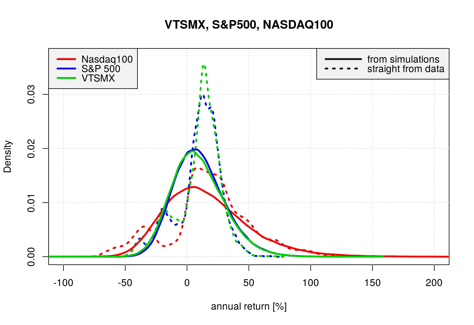

Time-series plots of returns

tmp <- dplyr::select(rr.df, date, time, VT, SP, NN) %>% 
              gather(. , name, value, NN, SP, VT)

ggplot(data = tmp, aes(x = date, y = value)) + theme_bw() + 
       theme(axis.title = element_text(size = 16),
             axis.text= element_text(size = 14),
             axis.line = element_line(size = 1),
             legend.position = c(0.9, 0.85)) +
       coord_cartesian(ylim = c(-75.0, 135.0)) +
       xlab("date") + 
       ylab("annualized returns") + 
       geom_hline(h=0, lty = 2, col = "orange") +
       geom_line(aes(color = name)) + 
       scale_colour_manual(values = c("red2", "blue2", "green4"), name = "Index", 
                           labels = c("NASDAQ100", "S&P500", "VTSMX"))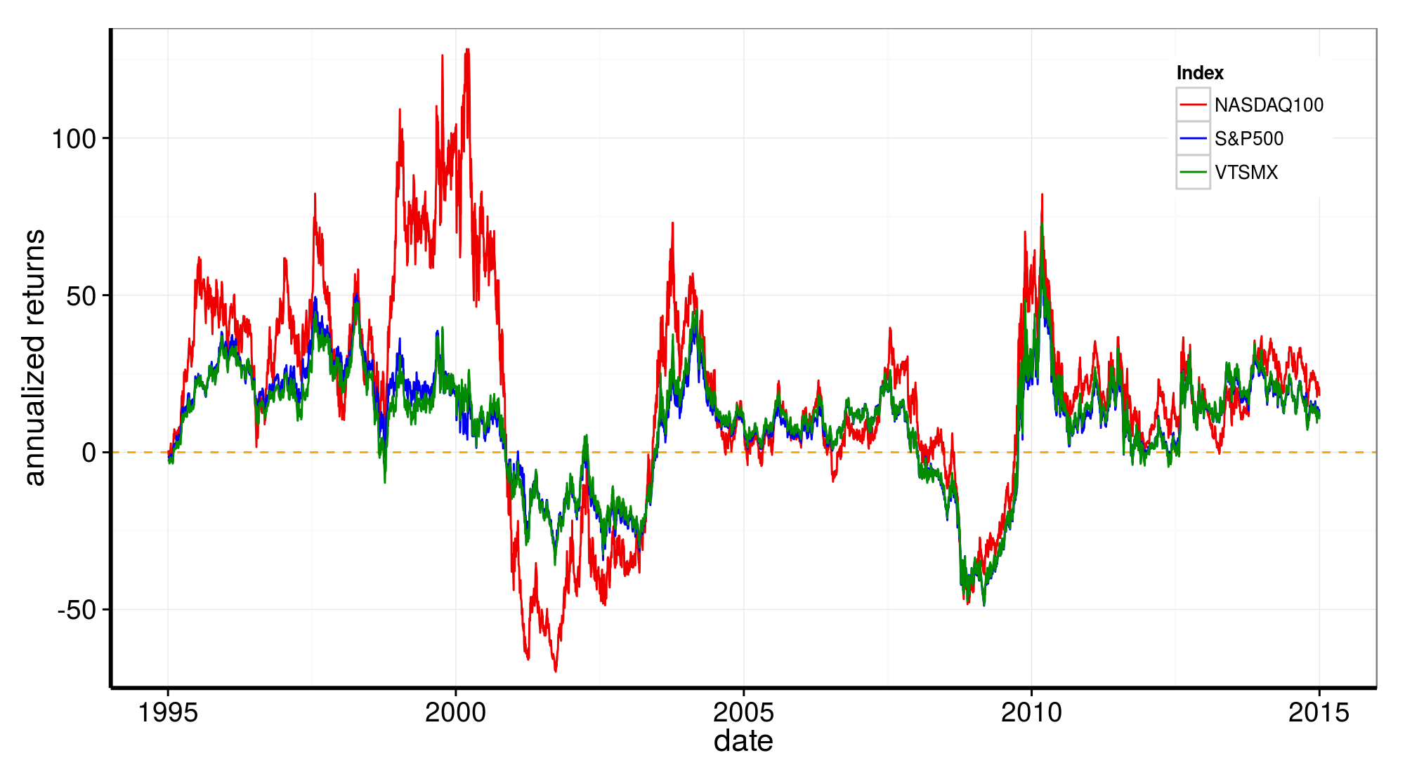

Time-series plots of indices (normalized to 1996-01-02)

tmp <- dplyr::select(rr.df, date, time, VTidx_n, SPidx_n, NNidx_n) %>% 
              gather(. , name, value, NNidx_n, SPidx_n, VTidx_n)

ggplot(data = tmp, aes(x = date, y = value)) + theme_bw() + 
       theme(axis.title = element_text(size = 16),
             axis.text= element_text(size = 14),
             axis.line = element_line(size = 1),
             legend.position = c(0.1, 0.85)) +
       xlab("date") + 
       ylab("indices (scaled to 1996-01-02)") + 
       scale_x_date(minor_breaks = "1 year") +
       scale_y_log10(breaks = c(1, 2, 4, 8)) +  
       geom_hline(h = 0, lty = 2, col = "orange") +
       geom_vline(xintercept = as.numeric(as.Date("1996-01-02")), lty = 2, col = "orange") +
       geom_line(aes(color = name)) + 
       scale_colour_manual(values = c("red2", "blue2", "green4"), name = "Index", 
                           labels = c("NASDAQ100", "S&P500", "VTSMX"))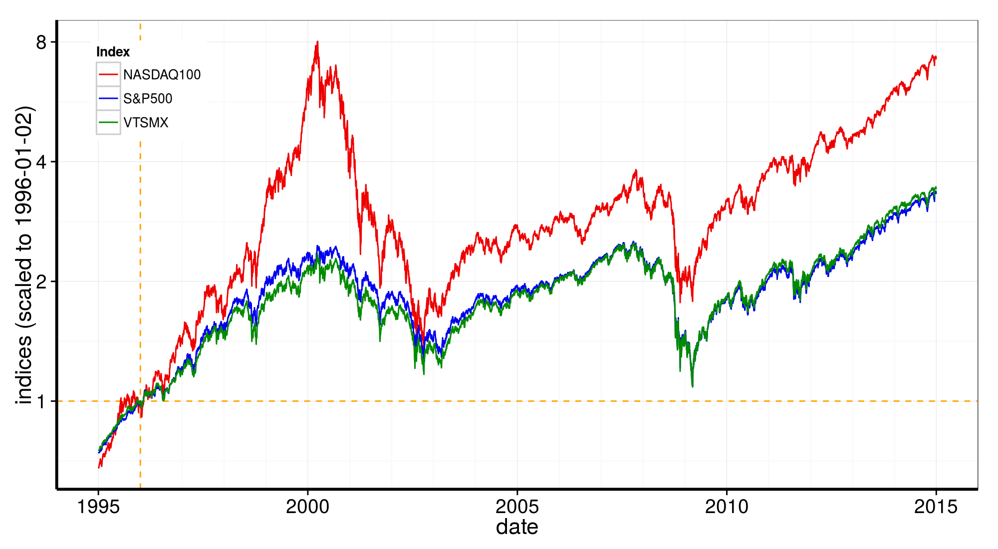

APPENDIX

Functions

Source code of the user-defined functions in scripts/my_functions_returns.R

#===================================================================================================

prepare_data <- function(data = NULL, xlin = NULL, xlog = NULL) {
    
    returns_log <- diff(log(data), lag = 1)
    returns_rel <- 100.0*(exp(returns_log) - 1)
    
    #---------------------------------------------------------------------
    # relative returns (linear, %)
    #---------------------------------------------------------------------

    # Fit with Generalized Lambda Distribution:
    rr_fit_gl <- fun.RMFMKL.ml(returns_rel)
    rr_fit_gl_y <- dgl(xlin, rr_fit_gl)

    # Fit with a Normal distribution, on the core of the data distribution
    rr_mean <- mean(returns_rel)
    rr_fit_norm1 <- fitdistr(returns_rel[abs(returns_rel - rr_mean) <= 5.0], "normal")
    rr_fit_norm2 <- fitdistr(returns_rel[abs(returns_rel - rr_mean) <= 2.0], "normal")

    rr_fit_norm1_y <- dnorm(xlin, mean = rr_fit_norm1$estimate[1], sd = rr_fit_norm1$estimate[2])
    rr_fit_norm2_y <- dnorm(xlin, mean = rr_fit_norm2$estimate[1], sd = rr_fit_norm2$estimate[2])

    rr_fit_n1 <- c(rr_fit_norm1$estimate[1], rr_fit_norm1$estimate[2])
    rr_fit_n2 <- c(rr_fit_norm2$estimate[1], rr_fit_norm2$estimate[2])

    returns_rel_distr.df <- data.frame(x = xlin, 
                                       y_gl = rr_fit_gl_y, 
                                       y_norm1 = rr_fit_norm1_y, 
                                       y_norm2 = rr_fit_norm2_y)

    #---------------------------------------------------------------------
    # log returns
    #---------------------------------------------------------------------

    # Fit with Generalized Lambda Distribution:
    rl_fit_gl <- fun.RMFMKL.ml(returns_log)
    rl_fit_gl_y <- dgl(xlog, rl_fit_gl)

    # Fit with a Normal distribution, on the core of the data distribution
    rl_mean <- mean(returns_log)
    rl_fit_norm1 <- fitdistr(returns_log[abs(returns_log - rl_mean) <= 0.05], "normal")
    rl_fit_norm2 <- fitdistr(returns_log[abs(returns_log - rl_mean) <= 0.02], "normal")

    rl_fit_norm1_y <- dnorm(xlog, mean = rl_fit_norm1$estimate[1], sd = rl_fit_norm1$estimate[2])
    rl_fit_norm2_y <- dnorm(xlog, mean = rl_fit_norm2$estimate[1], sd = rl_fit_norm2$estimate[2])
    
    rl_fit_n1 <- c(rl_fit_norm1$estimate[1], rl_fit_norm1$estimate[2])
    rl_fit_n2 <- c(rl_fit_norm2$estimate[1], rl_fit_norm2$estimate[2])
    
    returns_log_distr.df <- data.frame(x = xlog, 
                                       y_gl = rl_fit_gl_y, 
                                       y_norm1 = rl_fit_norm1_y, 
                                       y_norm2 = rl_fit_norm2_y)

    #---------------------------------------------------------------------

    list( rr_data = returns_rel,
          rr_fit_gl = rr_fit_gl,
          rr_fit_n1 = rr_fit_n1,
          rr_fit_n2 = rr_fit_n2,
          rr_distr = returns_rel_distr.df,
          rl_data = returns_log,
          rl_fit_gl = rl_fit_gl,
          rl_fit_n1 = rl_fit_n1,
          rl_fit_n2 = rl_fit_n2,
          rl_distr = returns_log_distr.df
        )
    
}

#===================================================================================================

mylog_trans <- function(base = exp(1), from = 0) {
    trans <- function(x) log(x, base) - from
    inv <- function(x) base^(x + from)
    trans_new("mylog", trans, inv, log_breaks(base = base), domain = c(base^from, Inf))
} 

#===================================================================================================

plot_distr_rel_returns <- function(data = NULL, 
                                   fits = NULL) {
    
    df <- data.frame(returns = data, stringsAsFactors = FALSE)

    pl.distr <- ggplot(data = df, aes(x = returns)) + theme_bw() + 
                    theme(axis.title = element_text(size = 16),
                          axis.text= element_text(size = 14),
                          axis.line = element_line(size = 1)) +
                    xlim(-8.0, 8.0) + 
                    xlab("daily relative returns (%)") + 
                    ylab("density") + 
                    geom_histogram(aes(y = ..density..), stat = "bin", drop = TRUE, 
                                   position = "identity", 
                                   binwidth = 0.2, 
                                   color = "grey50", fill = "gold", alpha = 0.3) + 
                    geom_line(data = fits, aes(x = x, y = y_norm1), color = "blue2", lty = 2, lwd = 1.5) + 
                    geom_line(data = fits, aes(x = x, y = y_norm2), color = "blue2", lwd = 1.5) + 
                    geom_line(data = fits, aes(x = x, y = y_gl), color = "red2", lwd = 1.5) + 
                    scale_y_continuous(trans = mylog_trans(base = 10, from = -3), 
                                       limits = c(0.001, 1.1), 
                                       breaks = c(0.001, 0.01, 0.1, 1.0))
    pl.distr

}

#===================================================================================================

plot_distr_log_returns <- function(data = NULL, 
                                   fits = NULL) {
    
    df <- data.frame(returns = data, stringsAsFactors = FALSE)
    hh <- hist(data, breaks = seq(-2.5, 2.5, by =0.0025), plot = FALSE)
    ymax <- 10.0**ceiling(log10(max(hh$density))) + 0.1

    pl.distr <- ggplot(data = df, aes(x = returns)) + theme_bw() + 
                    theme(axis.title = element_text(size = 16),
                          axis.text= element_text(size = 14),
                          axis.line = element_line(size = 1)) +
                    xlim(-0.1, 0.1) +
                    xlab("log(daily returns)") + 
                    ylab("density") + 
                    geom_histogram(aes(y = ..density..), stat = "bin", drop = TRUE, 
                                   position = "identity", 
                                   binwidth = 0.0025, 
                                   color = "grey50", fill = "gold", alpha = 0.3) + 
                    geom_line(data = fits, aes(x = x, y = y_norm1), color = "blue2", lty = 2, lwd = 1.5) + 
                    geom_line(data = fits, aes(x = x, y = y_norm2), color = "blue2", lwd = 1.5) + 
                    geom_line(data = fits, aes(x = x, y = y_gl), color = "red2", lwd = 1.5) +
                    scale_y_continuous(trans = mylog_trans(base = 10, from = -2),
                                       limits = c(0.01, ymax))
                                       # breaks = c(0.001, 0.01, 0.1, 1.0))

    pl.distr

}

#===================================================================================================

R Session Info

sessionInfo()
# R version 3.1.3 (2015-03-09)
# Platform: x86_64-pc-linux-gnu (64-bit)
# Running under: Ubuntu 14.04.2 LTS
# 
# locale:
#  [1] LC_CTYPE=en_US.UTF-8       LC_NUMERIC=C               LC_TIME=en_US.UTF-8       
#  [4] LC_COLLATE=C               LC_MONETARY=en_US.UTF-8    LC_MESSAGES=en_US.UTF-8   
#  [7] LC_PAPER=en_US.UTF-8       LC_NAME=C                  LC_ADDRESS=C              
# [10] LC_TELEPHONE=C             LC_MEASUREMENT=en_US.UTF-8 LC_IDENTIFICATION=C       
# 
# attached base packages:
# [1] grid      stats     graphics  grDevices utils     datasets  methods   base     
# 
# other attached packages:
#  [1] MASS_7.3-41     GLDEX_2.0.0.2   cluster_2.0.1   quantmod_0.4-4  TTR_0.22-0      xts_0.9-7      
#  [7] zoo_1.7-12      scales_0.2.4    gridExtra_0.9.1 ggplot2_1.0.1   tidyr_0.2.0     dplyr_0.4.2    
# [13] knitr_1.10.5   
# 
# loaded via a namespace (and not attached):
#  [1] DBI_0.3.1        R6_2.0.1         Rcpp_0.11.6      assertthat_0.1   codetools_0.2-11
#  [6] colorspace_1.2-6 digest_0.6.8     evaluate_0.7     formatR_1.2      gtable_0.1.2    
# [11] htmltools_0.2.6  labeling_0.3     lattice_0.20-31  lazyeval_0.1.10  magrittr_1.5    
# [16] munsell_0.4.2    parallel_3.1.3   plyr_1.8.3       proto_0.3-10     reshape2_1.4.1  
# [21] rmarkdown_0.7    stringi_0.5-5    stringr_1.0.0    tools_3.1.3      yaml_2.1.13

Stock Market Returns Distributions

Giovanni Fossati

Preliminaries

Introduction

Three Broad Market Indices : Daily Returns

Returns

Setup

Vanguard Total Stock Market Index

Distributions of relative returns and of log returns:

S&P 500

Distributions of relative returns and of log returns:

NASDAQ 100

Distributions of relative returns and of log returns:

Three Broad Market Indices : Annual Returns

Annual from Daily Returns

Annual straight from data

Time-series plots of returns

Time-series plots of indices (normalized to 1996-01-02)

APPENDIX

Functions

R Session Info